
Join 8,587 professionals who get data science tutorials, book recommendations, and tips/tricks each Saturday.
New to Python and SQL? I'll teach you both for free.
I won't send you spam. Unsubscribe at any time.
Issue #19 - Hierarchical Clustering Part 6: Cluster Distances
This Week’s Tutorial
You learned in Part 3 of this tutorial series how the agglomerative hierarchical clustering algorithm calculates the distance between two data points (i.e., rows) in a dataset.
You will learn in this week's tutorial the various methods the AgglomerativeClustering class from scikit-learn offers for calculating the distance between clusters.
As covered in Part 2 of this tutorial series, the algorithm needs both types of distances to mine the cluster hierarchy (i.e., taxonomy) from a dataset.
These methods for calculating distances between clusters are called linkages. The AgglomerativeClustering class supports four different linkages.
Understanding each linkage type is quite intuitive when you use a graphical representation. For this tutorial, assume we have the the following two clusters:

The first linkage is known as single link.
Single link calculates the distances between all the points in each of the clusters and then chooses the smallest of these distances to represent how similar (i.e., close together) the clusters are.
Graphically, single link would use the following two points for the distance between the clusters because it is the minimum:

Here's how to use single link with the AgglomerativeClustering class:

If there's a linkage that uses the minimum distance between two points in each cluster, it stands to reason that there would be a linkage that uses the maximum distance.
This is known as complete link.
I know.
Why couldn't they just call them min and max? 🤷♂️
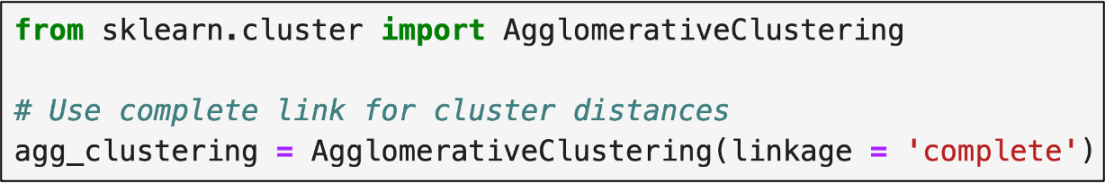
Here's complete link shown graphically:

And in code:
The next linkage is the average link. As you might have guessed, this linkage takes the average distance between all the data points for two clusters.
To keep the graphic from being overwhelming, I've only included the distance lines for two data points from the orange cluster:

Imagine all the distance lines from every data point in the orange cluster to every data point in the green cluster. The similarity of the clusters would be the average of all those distance lines, where a smaller average indicates more similar clusters.
Here's the code to specify using average link:

The last linkage is the AgglomerativeClustering default - the ward linkage. The ward linkage (or Ward's method) is more involved than the previous linkages.
If you're familiar with the k-means clustering algorithm (e.g., from my Cluster Analysis with Python online course), then ward linkage will be familiar to you.
The ward linkage uses what are known as prototypes. Think of prototypes as being data points the algorithm "makes up" to be the center of each cluster.
The most common type of prototype is a centroid which is defined as the average of all the data points in the cluster.
Graphically, the orange and green dots are the centroids of the two clusters in our running example:

The ward linkage first evaluates each cluster by finding all the distances (i.e., the dotted lines) between the data points in a cluster and their centroid:

Consider the orange cluster above. There are eight data points in the cluster and eight distances between each data point and the centroid.
The ward linkage takes each one of these distance values and squares them (i.e., the distance multiplied by itself). It then adds all these squared distances together.
It then repeats this process for the green cluster.
Lastly, it then adds the sum of the squared distances for the orange cluster to the sum of the squared distances for the green cluster.
Think of this last calculation (i.e., adding the two sums together) as being the baseline.
The ward linkage then combines the two clusters and calculates a new centroid (represented in blue):

The ward linkage then sums up all the squared distances for the new, larger cluster:

Think of the sum of the squared distances for the new, larger cluster as being the new hotness.
Ward linkage calculates the difference between the baseline and the new hotness and treats this as a penalty for combining clusters. Ward linkage looks to make this penalty as small as possible when considering which clusters to combine.
By minimizing the penalty, ward linkage prioritizes combining clusters that are most similar.
Even though Ward's method is the default, here's the code for reference:

It shouldn't come as a surprise that using different linkages can produce different clusterings.
So, you may be asking yourself, "which linkage should I use?"
When it comes to cluster analysis, I'm a big fan of experimenting to see what works the best. For example, using different linkages and see which produces the most useful clusters.
That being said, here are some rules of thumb:
Single link is good at handling non-spherical cluster shapes, but is sensitive to outliers.
Complete link is less susceptible to outliers, but can break large clusters and it tends to produce spherical clusters.
Think of average link as being a compromise between single and complete linkages.
Think of Ward's method as being a bit of an improvement over average link.
This Week’s Book
I regularly teach text analytics with Python as part of my live Machine Learning Bootcamps. This course leverages the power of the Natural Language Toolkit (NLTK).
If you're not familiar with the NLTK, it is a Python library designed for working with text data (e.g., customer service chats). The library authors did the community a solid and offer a free online version of their book:

So many organizations are suffering from Generative AI FOMO. What they should really be focusing on is how to use battle-tested techniques that work with the realities of their data.
Text analytics with the NLTK is one of those battle-tested techniques.
That's it for this week.
Stay tuned for next week's newsletter which will be the last in this series. The topic is using ML predictive models to help interpret clusters.
Stay healthy and happy data sleuthing!

Dave Langer
Whenever you're ready, there are 4 ways I can help you:
1 - Are you new to data analysis? My Visual Analysis with Python online course will teach you the fundamentals you need - fast. No complex math required, and it works with Python in Excel!
2 - Cluster Analysis with Python: Most of the world's data is unlabeled and can't be used for predictive models. This is where my self-paced online course teaches you how to extract insights from your unlabeled data.
3 - Introduction to Machine Learning: This self-paced online course teaches you how to build predictive models like regression trees and the mighty random forest using Python. Offered in partnership with TDWI, use code LANGER to save 20% off.
4 - Is machine learning right for your business, but don't know where to start? Check out my Machine Learning Accelerator.